microgpt · MarketNews

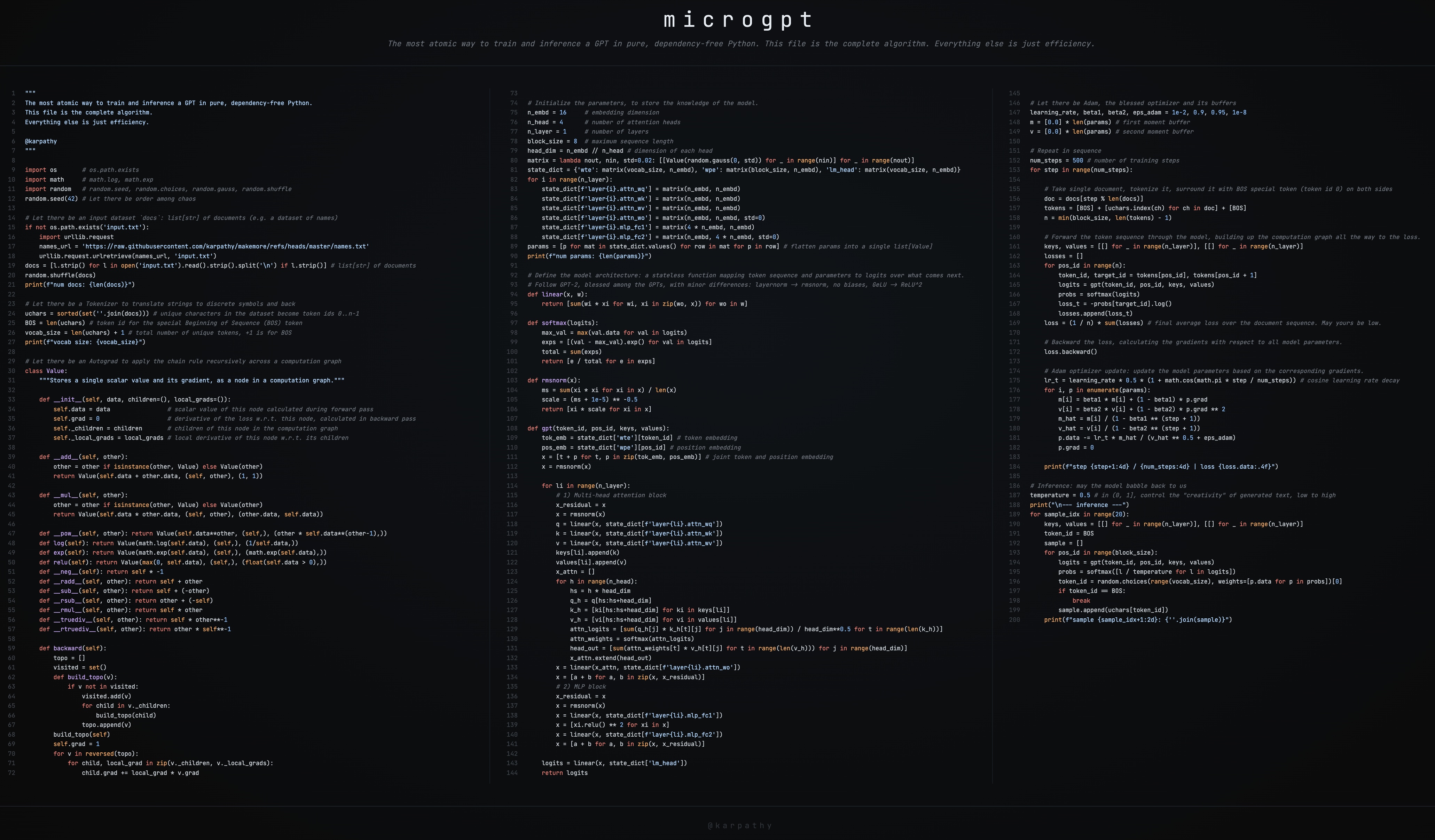
This is a brief guide to my new art project microgpt, a single file of 200 lines of pure Python with no dependencies that trains and inferences a GPT. This file contains the full algorithmic content of what is needed: dataset of documents, tokenizer, autograd engine, a GPT-2-like neural network architecture, the Adam optimizer, training loop, and inference loop. Everything else is just efficiency. I cannot simplify this any further. This script is the culmination of multiple projects (micrograd, makemore, nanogpt, etc.) and a decade-long obsession to simplify LLMs to their bare essentials, and I think it is beautiful 🥹. It even breaks perfectly across 3 columns:

Это краткий гид по моему новому арт-проекту microgpt — одному файлу в 200 строк чистого Python без зависимостей, который обучает GPT и запускает её инференс. В этом файле содержится всё алгоритмически необходимое: датасет документов, токенизатор, движок autograd, нейросетевая архитектура в духе GPT-2, оптимизатор Adam, цикл обучения и цикл инференса. Всё остальное — это лишь вопросы эффективности. Упростить дальше я уже не могу. Этот скрипт — кульминация нескольких проектов (micrograd, makemore, nanogpt и др.) и десятилетней одержимости свести LLM к их сути, и я считаю, что это красиво 🥹. Он даже идеально разбивается на 3 колонки:

Where to find it:

Где найти:

This GitHub gist has the full source code: microgpt.py

It’s also available on this web page: https://karpathy.ai/microgpt.html

Also available as a Google Colab notebook

NEW: buy microgpt as a triptych on my art store at karpathy.art :)

В этом GitHub gist лежит весь исходный код: microgpt.py. Также доступен на этой веб-странице: https://karpathy.ai/microgpt.html. И в виде Google Colab notebook. NEW: купить microgpt как триптих можно в моём арт-магазине karpathy.art :)

The following is my guide on stepping an interested reader through the code.

Далее — мой гид, который проведёт заинтересованного читателя по коду.

Dataset

Датасет

The fuel of large language models is a stream of text data, optionally separated into a set of documents. In production-grade applications, each document would be an internet web page but for microgpt we use a simpler example of 32,000 names, one per line:

Топливо больших языковых моделей — поток текстовых данных, опционально разделённый на набор документов. В промышленных приложениях каждый документ — это веб-страница из интернета, но для microgpt мы используем более простой пример: 32 000 имён по одному на строку:

# Let there be an input dataset `docs`: list[str] of documents (e.g. a dataset of names) if not os.path.exists('input.txt'): import urllib.request names_url = 'https://raw.githubusercontent.com/karpathy/makemore/refs/heads/master/names.txt' urllib.request.urlretrieve(names_url, 'input.txt') docs = [l.strip() for l in open('input.txt').read().strip().split('\n') if l.strip()] # list[str] of documents random.shuffle(docs) print(f"num docs: {len(docs)}")

# Пусть есть входной датасет `docs`: list[str] документов (например, датасет имён) if not os.path.exists('input.txt'): import urllib.request names_url = 'https://raw.githubusercontent.com/karpathy/makemore/refs/heads/master/names.txt' urllib.request.urlretrieve(names_url, 'input.txt') docs = [l.strip() for l in open('input.txt').read().strip().split('\n') if l.strip()] # list[str] документов random.shuffle(docs) print(f"num docs: {len(docs)}")

The dataset looks like this. Each name is a document:

Датасет выглядит так. Каждое имя — это документ:

emma olivia ava isabella sophia charlotte mia amelia harper ... (~32,000 names follow)

emma olivia ava isabella sophia charlotte mia amelia harper ... (далее ~32 000 имён)

The goal of the model is to learn the patterns in the data and then generate similar new documents that share the statistical patterns within. As a preview, by the end of the script our model will generate (“hallucinate”!) new, plausible-sounding names. Skipping ahead, we’ll get:

Цель модели — выучить закономерности в данных и затем генерировать похожие новые документы, которые разделяют те же статистические паттерны. В качестве превью: к концу скрипта наша модель будет генерировать («галлюцинировать»!) новые правдоподобно звучащие имена. Забегая вперёд, мы получим:

sample 1: kamon sample 2: ann sample 3: karai sample 4: jaire sample 5: vialan sample 6: karia sample 7: yeran sample 8: anna sample 9: areli sample 10: kaina sample 11: konna sample 12: keylen sample 13: liole sample 14: alerin sample 15: earan sample 16: lenne sample 17: kana sample 18: lara sample 19: alela sample 20: anton

It doesn’t look like much, but from the perspective of a model like ChatGPT, your conversation with it is just a funny looking “document”. When you initialize the document with your prompt, the model’s response from its perspective is just a statistical document completion.

Выглядит не слишком впечатляюще, но с точки зрения модели вроде ChatGPT ваш диалог с ней — это просто странновато выглядящий «документ». Когда вы инициализируете документ своим промптом, ответ модели с её точки зрения — это просто статистическое продолжение документа.

Tokenizer

Токенизатор

Under the hood, neural networks work with numbers, not characters, so we need a way to convert text into a sequence of integer token ids and back. Production tokenizers like tiktoken (used by GPT-4) operate on chunks of characters for efficiency, but the simplest possible tokenizer just assigns one integer to each unique character in the dataset:

Под капотом нейросети работают с числами, а не с символами, поэтому нам нужен способ конвертировать текст в последовательность целочисленных id токенов и обратно. Промышленные токенизаторы вроде tiktoken (используется GPT-4) для эффективности оперируют группами символов, но простейший возможный токенизатор просто присваивает по одному целому числу каждому уникальному символу в датасете:

# Let there be a Tokenizer to translate strings to discrete symbols and back uchars = sorted(set(''.join(docs))) # unique characters in the dataset become token ids 0..n-1 BOS = len(uchars) # token id for the special Beginning of Sequence (BOS) token vocab_size = len(uchars) + 1 # total number of unique tokens, +1 is for BOS print(f"vocab size: {vocab_size}")

# Пусть есть Tokenizer для перевода строк в дискретные символы и обратно uchars = sorted(set(''.join(docs))) # уникальные символы в датасете становятся id токенов 0..n-1 BOS = len(uchars) # id специального токена Beginning of Sequence (BOS) vocab_size = len(uchars) + 1 # общее число уникальных токенов, +1 — это BOS print(f"vocab size: {vocab_size}")

In the code above, we collect all unique characters across the dataset (which are just all the lowercase letters a-z), sort them, and each letter gets an id by its index. Note that the integer values themselves have no meaning at all; each token is just a separate discrete symbol. Instead of 0, 1, 2 they might as well be different emoji. In addition, we create one more special token called BOS (Beginning of Sequence), which acts as a delimiter: it tells the model “a new document starts/ends here”. Later during training, each document gets wrapped with BOS on both sides: [BOS, e, m, m, a, BOS]. The model learns that BOS initates a new name, and that another BOS ends it. Therefore, we have a final vocavulary of 27 (26 possible lowercase characters a-z and +1 for the BOS token).

В коде выше мы собираем все уникальные символы по датасету (это просто все строчные буквы a-z), сортируем их, и каждая буква получает id по своему индексу. Заметьте, что сами целочисленные значения не имеют никакого смысла; каждый токен — это просто отдельный дискретный символ. Вместо 0, 1, 2 это вполне могли бы быть разные эмодзи. Кроме того, мы создаём ещё один специальный токен под названием BOS (Beginning of Sequence), который служит разделителем: он говорит модели «здесь начинается/заканчивается новый документ». Позже во время обучения каждый документ оборачивается BOS с обеих сторон: [BOS, e, m, m, a, BOS]. Модель учится тому, что BOS начинает новое имя, а следующий BOS его заканчивает. Итого мы получаем финальный словарь из 27 элементов (26 возможных строчных символов a-z плюс токен BOS).

Autograd

Training a neural network requires gradients: for each parameter in the model, we need to know “if I nudge this number up a little, does the loss go up or down, and by how much?”. The computation graph has many inputs (the model parameters and the input tokens) but funnels down to a single scalar output: the loss (we’ll define exactly what the loss is below). Backpropagation starts at that single output and works backwards through the graph, computing the gradient of the loss with respect to every input. It relies on the chain rule from calculus. In production, libraries like PyTorch handle this automatically. Here, we implement it from scratch in a single class called Value:

Для обучения нейросети нужны градиенты: для каждого параметра модели нам надо знать «если я чуть-чуть увеличу это число, loss вырастет или упадёт, и насколько?». У вычислительного графа много входов (параметры модели и входные токены), но он сходится к одному скалярному выходу: loss (мы определим, что такое loss, ниже). Backpropagation начинается с этого единственного выхода и движется в обратную сторону по графу, вычисляя градиент loss по каждому входу. Он опирается на цепное правило из матанализа. В промышленных решениях это автоматически делают библиотеки вроде PyTorch. Здесь мы реализуем его с нуля в одном классе под названием Value:

class Value: __slots__ = ('data', 'grad', '_children', '_local_grads') def __init__(self, data, children=(), local_grads=()): self.data = data # scalar value of this node calculated during forward pass self.grad = 0 # derivative of the loss w.r.t. this node, calculated in backward pass self._children = children # children of this node in the computation graph self._local_grads = local_grads # local derivative of this node w.r.t. its children def __add__(self, other): other = other if isinstance(other, Value) else Value(other) return Value(self.data + other.data, (self, other), (1, 1)) def __mul__(self, other): other = other if isinstance(other, Value) else Value(other) return Value(self.data * other.data, (self, other), (other.data, self.data)) def __pow__(self, other): return Value(self.data**other, (self,), (other * self.data**(other-1),)) def log(self): return Value(math.log(self.data), (self,), (1/self.data,)) def exp(self): return Value(math.exp(self.data), (self,), (math.exp(self.data),)) def relu(self): return Value(max(0, self.data), (self,), (float(self.data > 0),)) def __neg__(self): return self * -1 def __radd__(self, other): return self + other def __sub__(self, other): return self + (-other) def __rsub__(self, other): return other + (-self) def __rmul__(self, other): return self * other def __truediv__(self, other): return self * other**-1 def __rtruediv__(self, other): return other * self**-1 def backward(self): topo = [] visited = set() def build_topo(v): if v not in visited: visited.add(v) for child in v._children: build_topo(child) topo.append(v) build_topo(self) self.grad = 1 for v in reversed(topo): for child, local_grad in zip(v._children, v._local_grads): child.grad += local_grad * v.grad

class Value: __slots__ = ('data', 'grad', '_children', '_local_grads') def __init__(self, data, children=(), local_grads=()): self.data = data # скалярное значение этого узла, посчитанное при forward pass self.grad = 0 # производная loss по этому узлу, считается при backward pass self._children = children # дети этого узла в вычислительном графе self._local_grads = local_grads # локальная производная этого узла по его детям def __add__(self, other): other = other if isinstance(other, Value) else Value(other) return Value(self.data + other.data, (self, other), (1, 1)) def __mul__(self, other): other = other if isinstance(other, Value) else Value(other) return Value(self.data * other.data, (self, other), (other.data, self.data)) def __pow__(self, other): return Value(self.data**other, (self,), (other * self.data**(other-1),)) def log(self): return Value(math.log(self.data), (self,), (1/self.data,)) def exp(self): return Value(math.exp(self.data), (self,), (math.exp(self.data),)) def relu(self): return Value(max(0, self.data), (self,), (float(self.data > 0),)) def __neg__(self): return self * -1 def __radd__(self, other): return self + other def __sub__(self, other): return self + (-other) def __rsub__(self, other): return other + (-self) def __rmul__(self, other): return self * other def __truediv__(self, other): return self * other**-1 def __rtruediv__(self, other): return other * self**-1 def backward(self): topo = [] visited = set() def build_topo(v): if v not in visited: visited.add(v) for child in v._children: build_topo(child) topo.append(v) build_topo(self) self.grad = 1 for v in reversed(topo): for child, local_grad in zip(v._children, v._local_grads): child.grad += local_grad * v.grad

I realize that this is the most mathematically and algorithmically intense part and I have a 2.5 hour video on it: micrograd video. Briefly, a Value wraps a single scalar number (.data) and tracks how it was computed. Think of each operation as a little lego block: it takes some inputs, produces an output (the forward pass), and it knows how its output would change with respect to each of its inputs (the local gradient). That’s all the information autograd needs from each block. Everything else is just the chain rule, stringing the blocks together.

Я понимаю, что это самая математически и алгоритмически насыщенная часть, и у меня есть 2,5-часовое видео по ней: видео про micrograd. Если коротко, Value оборачивает одно скалярное число (.data) и отслеживает, как оно было получено. Представьте каждую операцию как маленький лего-блок: он принимает на вход какие-то входы, выдаёт выход (forward pass) и знает, как его выход изменится по отношению к каждому из входов (локальный градиент). Это вся информация, которая нужна autograd от каждого блока. Всё остальное — это просто цепное правило, нанизывающее блоки друг на друга.

Every time you do math with Value objects (add, multiply, etc.), the result is a new Value that remembers its inputs (_children) and the local derivative of that operation (_local_grads). For example, __mul__ records that \(\frac{\partial(a \cdot b)}{\partial a} = b\) and \(\frac{\partial(a \cdot b)}{\partial b} = a\). The full set of lego blocks:

Каждый раз, когда вы делаете математику над объектами Value (сложение, умножение и т. д.), результатом становится новый Value, помнящий свои входы (_children) и локальную производную этой операции (_local_grads). Например, __mul__ запоминает, что \(\frac{\partial(a \cdot b)}{\partial a} = b\) и \(\frac{\partial(a \cdot b)}{\partial b} = a\). Полный набор лего-блоков:

The backward() method walks this graph in reverse topological order (starting from the loss, ending at the parameters), applying the chain rule at each step. If the loss is \(L\) and a node \(v\) has a child \(c\) with local gradient \(\frac{\partial v}{\partial c}\), then:

Метод backward() обходит этот граф в обратном топологическом порядке (начиная от loss и заканчивая параметрами), применяя цепное правило на каждом шаге. Если loss обозначить как \(L\), а у узла \(v\) есть ребёнок \(c\) с локальным градиентом \(\frac{\partial v}{\partial c}\), то:

This looks a bit scary if you’re not comfortable with your calculus, but this is literally just multiplying two numbers in an intuitive way. One way to see it looks as follows: “If a car travels twice as fast as a bicycle and the bicycle is four times as fast as a walking man, then the car travels 2 x 4 = 8 times as fast as the man.” The chain rule is the same idea: you multiply the rates of change along the path.

Это выглядит слегка пугающе, если вы не очень в ладах с матанализом, но на самом деле тут просто перемножаются два числа интуитивным образом. Один из способов это увидеть: «Если машина едет в два раза быстрее велосипеда, а велосипед — в четыре раза быстрее идущего человека, то машина едет в 2 × 4 = 8 раз быстрее человека». Цепное правило — это та же идея: вы перемножаете скорости изменения вдоль пути.

We kick things off by setting self.grad = 1 at the loss node, because \(\frac{\partial L}{\partial L} = 1\): the loss’s rate of change with respect to itself is trivially 1. From there, the chain rule just multiplies local gradients along every path back to the parameters.

Запускаем всё, выставив self.grad = 1 на узле loss, потому что \(\frac{\partial L}{\partial L} = 1\): скорость изменения loss по самому себе тривиально равна 1. Дальше цепное правило просто перемножает локальные градиенты вдоль каждого пути обратно к параметрам.

Note the += (accumulation, not assignment). When a value is used in multiple places in the graph (i.e. the graph branches), gradients flow back along each branch independently and must be summed. This is a consequence of the multivariable chain rule: if \(c\) contributes to \(L\) through multiple paths, the total derivative is the sum of contributions from each path.

Обратите внимание на += (накопление, а не присваивание). Когда значение используется в нескольких местах графа (т. е. граф ветвится), градиенты текут обратно по каждой ветке независимо и должны суммироваться. Это следствие многомерного цепного правила: если \(c\) вносит вклад в \(L\) по нескольким путям, общая производная — это сумма вкладов от каждого пути.

After backward() completes, every Value in the graph has a .grad containing \(\frac{\partial L}{\partial v}\), which tells us how the final loss would change if we nudged that value.

После завершения backward() у каждого Value в графе есть .grad, содержащий \(\frac{\partial L}{\partial v}\), который говорит нам, как изменился бы итоговый loss, если бы мы чуть подёргали это значение.

Here’s a concrete example. Note that a is used twice (the graph branches), so its gradient is the sum of both paths:

Вот конкретный пример. Заметьте, что a используется дважды (граф ветвится), поэтому её градиент — сумма по обоим путям:

a = Value(2.0) b = Value(3.0) c = a * b # c = 6.0 L = c + a # L = 8.0 L.backward() print(a.grad) # 4.0 (dL/da = b + 1 = 3 + 1, via both paths) print(b.grad) # 2.0 (dL/db = a = 2)

a = Value(2.0) b = Value(3.0) c = a * b # c = 6.0 L = c + a # L = 8.0 L.backward() print(a.grad) # 4.0 (dL/da = b + 1 = 3 + 1, по обоим путям) print(b.grad) # 2.0 (dL/db = a = 2)

This is exactly what PyTorch’s .backward() gives you:

Ровно это же даёт .backward() в PyTorch:

import torch a = torch.tensor(2.0, requires_grad=True) b = torch.tensor(3.0, requires_grad=True) c = a * b L = c + a L.backward() print(a.grad) # tensor(4.) print(b.grad) # tensor(2.)

This is the same algorithm that PyTorch’s loss.backward() runs, just on scalars instead of tensors (arrays of scalars) - algorithmically identical, significantly smaller and simpler, but of course a lot less efficient.

Это тот же алгоритм, который выполняет loss.backward() в PyTorch, только на скалярах, а не на тензорах (массивах скаляров) — алгоритмически идентично, существенно меньше и проще, но, разумеется, заметно менее эффективно.

Let’s spell what the .backward() gives us above. Autograd calculated that if L = a*b + a, and a=2 and b=3, then a.grad = 4.0 is telling us about the local influence of a on L. If you wiggle the inmput a, in what direction is L changing? Here, the derivative of L w.r.t. a is 4.0, meaning that if we increase a by a tiny amount (say 0.001), L would increase by about 4x that (0.004). Similarly, b.grad = 2.0 means the same nudge to b would increase L by about 2x that (0.002). In other words, these gradients tell us the direction (positive or negative depending on the sign), and the steepness (the magnitude) of the influence of each individual input on the final output (the loss). This then allows us to interately nudge the parameters of our neural network to lower the loss, and hence improve its predictions.

Давайте раскроем то, что нам выше дал .backward(). Autograd посчитал, что если L = a*b + a, и a=2, и b=3, то a.grad = 4.0 говорит нам о локальном влиянии a на L. Если вы пошевелите вход a, в какую сторону изменится L? Здесь производная L по a равна 4.0, то есть если мы увеличим a на крошечную величину (скажем, 0.001), L увеличится примерно в 4 раза больше (0.004). Аналогично b.grad = 2.0 означает, что такое же подталкивание b увеличило бы L примерно вдвое больше этой величины (0.002). Иначе говоря, эти градиенты сообщают нам направление (положительное или отрицательное в зависимости от знака) и крутизну (величину) влияния каждого отдельного входа на итоговый выход (loss). Это и позволяет нам итеративно подталкивать параметры нашей нейросети, чтобы снижать loss и тем самым улучшать её предсказания.

Parameters

Параметры

The parameters are the knowledge of the model. They are a large collection of floating point numbers (wrapped in Value for autograd) that start out random and are iteratively optimized during training. The exact role of each parameter will make more sense once we define the model architecture below, but for now we just need to initialize them:

Параметры — это знания модели. Это большой набор чисел с плавающей точкой (обёрнутых в Value для autograd), которые начинаются как случайные и итеративно оптимизируются во время обучения. Точная роль каждого параметра станет понятнее, когда мы определим архитектуру модели ниже, но пока нам надо лишь их инициализировать:

n_embd = 16 # embedding dimension n_head = 4 # number of attention heads n_layer = 1 # number of layers block_size = 16 # maximum sequence length head_dim = n_embd // n_head # dimension of each head matrix = lambda nout, nin, std=0.08: [[Value(random.gauss(0, std)) for _ in range(nin)] for _ in range(nout)] state_dict = {'wte': matrix(vocab_size, n_embd), 'wpe': matrix(block_size, n_embd), 'lm_head': matrix(vocab_size, n_embd)} for i in range(n_layer): state_dict[f'layer{i}.attn_wq'] = matrix(n_embd, n_embd) state_dict[f'layer{i}.attn_wk'] = matrix(n_embd, n_embd) state_dict[f'layer{i}.attn_wv'] = matrix(n_embd, n_embd) state_dict[f'layer{i}.attn_wo'] = matrix(n_embd, n_embd) state_dict[f'layer{i}.mlp_fc1'] = matrix(4 * n_embd, n_embd) state_dict[f'layer{i}.mlp_fc2'] = matrix(n_embd, 4 * n_embd) params = [p for mat in state_dict.values() for row in mat for p in row] print(f"num params: {len(params)}")

n_embd = 16 # размерность эмбеддинга n_head = 4 # число attention-голов n_layer = 1 # число слоёв block_size = 16 # максимальная длина последовательности head_dim = n_embd // n_head # размерность каждой головы matrix = lambda nout, nin, std=0.08: [[Value(random.gauss(0, std)) for _ in range(nin)] for _ in range(nout)] state_dict = {'wte': matrix(vocab_size, n_embd), 'wpe': matrix(block_size, n_embd), 'lm_head': matrix(vocab_size, n_embd)} for i in range(n_layer): state_dict[f'layer{i}.attn_wq'] = matrix(n_embd, n_embd) state_dict[f'layer{i}.attn_wk'] = matrix(n_embd, n_embd) state_dict[f'layer{i}.attn_wv'] = matrix(n_embd, n_embd) state_dict[f'layer{i}.attn_wo'] = matrix(n_embd, n_embd) state_dict[f'layer{i}.mlp_fc1'] = matrix(4 * n_embd, n_embd) state_dict[f'layer{i}.mlp_fc2'] = matrix(n_embd, 4 * n_embd) params = [p for mat in state_dict.values() for row in mat for p in row] print(f"num params: {len(params)}")

Each parameter is initialized to a small random number drawn from a Gaussian distribution. The state_dict organizes them into named matrices (borrowing PyTorch’s terminology): embedding tables, attention weights, MLP weights, and a final output projection. We also flatten all parameters into a single list params so the optimizer can loop over them later. In our tiny model this comes out to 4,192 parameters. GPT-2 had 1.6 billion, and modern LLMs have hundreds of billions.

Каждый параметр инициализируется небольшим случайным числом из гауссовского распределения. state_dict организует их в именованные матрицы (заимствуя терминологию PyTorch): таблицы эмбеддингов, веса attention, веса MLP и финальная выходная проекция. Также мы складываем все параметры в один плоский список params, чтобы оптимизатору потом было удобно по ним пройтись. В нашей крошечной модели получается 4192 параметра. У GPT-2 было 1,6 миллиарда, а у современных LLM — сотни миллиардов.

Architecture

Архитектура

The model architecture is a stateless function: it takes a token, a position, the parameters, and the cached keys/values from previous positions, and returns logits (scores) over what token the model things should come next in the sequence. We follow GPT-2 with minor simplifications: RMSNorm instead of LayerNorm, no biases, and ReLU instead of GeLU. First, three small helper functions:

Архитектура модели — это функция без состояния: она принимает токен, позицию, параметры и закэшированные keys/values с предыдущих позиций, и возвращает logits (оценки) того, какой токен, по мнению модели, должен идти следующим в последовательности. Мы следуем GPT-2 с небольшими упрощениями: RMSNorm вместо LayerNorm, без bias-ов и ReLU вместо GeLU. Сначала три маленькие вспомогательные функции:

def linear(x, w): return [sum(wi * xi for wi, xi in zip(wo, x)) for wo in w]

linear is a matrix-vector multiply. It takes a vector x and a weight matrix w, and computes one dot product per row of w. This is the fundamental building block of neural networks: a learned linear transformation.

linear — это умножение матрицы на вектор. Она принимает вектор x и матрицу весов w и вычисляет по одному скалярному произведению на каждую строку w. Это фундаментальный строительный блок нейросетей: обучаемое линейное преобразование.

def softmax(logits): max_val = max(val.data for val in logits) exps = [(val - max_val).exp() for val in logits] total = sum(exps) return [e / total for e in exps]

softmax converts a vector of raw scores (logits), which can range from \(-\infty\) to \(+\infty\), into a probability distribution: all values end up in \([0, 1]\) and sum to 1. We subtract the max first for numerical stability (it doesn’t change the result mathematically, but prevents overflow in exp).

softmax переводит вектор сырых оценок (logits), которые могут лежать в диапазоне от \(-\infty\) до \(+\infty\), в распределение вероятностей: все значения оказываются в \([0, 1]\) и в сумме дают 1. Сначала мы вычитаем максимум для численной устойчивости (математически это не меняет результат, но предотвращает переполнение в exp).

def rmsnorm(x): ms = sum(xi * xi for xi in x) / len(x) scale = (ms + 1e-5) ** -0.5 return [xi * scale for xi in x]

rmsnorm (Root Mean Square Normalization) rescales a vector so its values have unit root-mean-square. This keeps activations from growing or shrinking as they flow through the network, which stabilizes training. It’s a simpler variant of the LayerNorm used in the original GPT-2.

rmsnorm (Root Mean Square Normalization) перенормирует вектор так, чтобы его значения имели единичное среднеквадратичное значение. Это удерживает активации от взрывного роста или затухания по мере прохождения через сеть, что стабилизирует обучение. Это более простой вариант LayerNorm, использовавшегося в оригинальной GPT-2.

Now the model itself:

Теперь сама модель:

def gpt(token_id, pos_id, keys, values): tok_emb = state_dict['wte'][token_id] # token embedding pos_emb = state_dict['wpe'][pos_id] # position embedding x = [t + p for t, p in zip(tok_emb, pos_emb)] # joint token and position embedding x = rmsnorm(x) for li in range(n_layer): # 1) Multi-head attention block x_residual = x x = rmsnorm(x) q = linear(x, state_dict[f'layer{li}.attn_wq']) k = linear(x, state_dict[f'layer{li}.attn_wk']) v = linear(x, state_dict[f'layer{li}.attn_wv']) keys[li].append(k) values[li].append(v) x_attn = [] for h in range(n_head): hs = h * head_dim q_h = q[hs:hs+head_dim] k_h = [ki[hs:hs+head_dim] for ki in keys[li]] v_h = [vi[hs:hs+head_dim] for vi in values[li]] attn_logits = [sum(q_h[j] * k_h[t][j] for j in range(head_dim)) / head_dim**0.5 for t in range(len(k_h))] attn_weights = softmax(attn_logits) head_out = [sum(attn_weights[t] * v_h[t][j] for t in range(len(v_h))) for j in range(head_dim)] x_attn.extend(head_out) x = linear(x_attn, state_dict[f'layer{li}.attn_wo']) x = [a + b for a, b in zip(x, x_residual)] # 2) MLP block x_residual = x x = rmsnorm(x) x = linear(x, state_dict[f'layer{li}.mlp_fc1']) x = [xi.relu() for xi in x] x = linear(x, state_dict[f'layer{li}.mlp_fc2']) x = [a + b for a, b in zip(x, x_residual)] logits = linear(x, state_dict['lm_head']) return logits

def gpt(token_id, pos_id, keys, values): tok_emb = state_dict['wte'][token_id] # эмбеддинг токена pos_emb = state_dict['wpe'][pos_id] # эмбеддинг позиции x = [t + p for t, p in zip(tok_emb, pos_emb)] # совместный эмбеддинг токена и позиции x = rmsnorm(x) for li in range(n_layer): # 1) Multi-head attention block x_residual = x x = rmsnorm(x) q = linear(x, state_dict[f'layer{li}.attn_wq']) k = linear(x, state_dict[f'layer{li}.attn_wk']) v = linear(x, state_dict[f'layer{li}.attn_wv']) keys[li].append(k) values[li].append(v) x_attn = [] for h in range(n_head): hs = h * head_dim q_h = q[hs:hs+head_dim] k_h = [ki[hs:hs+head_dim] for ki in keys[li]] v_h = [vi[hs:hs+head_dim] for vi in values[li]] attn_logits = [sum(q_h[j] * k_h[t][j] for j in range(head_dim)) / head_dim**0.5 for t in range(len(k_h))] attn_weights = softmax(attn_logits) head_out = [sum(attn_weights[t] * v_h[t][j] for t in range(len(v_h))) for j in range(head_dim)] x_attn.extend(head_out) x = linear(x_attn, state_dict[f'layer{li}.attn_wo']) x = [a + b for a, b in zip(x, x_residual)] # 2) MLP block x_residual = x x = rmsnorm(x) x = linear(x, state_dict[f'layer{li}.mlp_fc1']) x = [xi.relu() for xi in x] x = linear(x, state_dict[f'layer{li}.mlp_fc2']) x = [a + b for a, b in zip(x, x_residual)] logits = linear(x, state_dict['lm_head']) return logits

The function processes one token (of id token_id) at a specific position in time (pos_id), and some context from the previous iterations summarized by the activations in keys and values, known as the KV Cache. Here’s what happens step by step:

Функция обрабатывает один токен (с id token_id) в конкретной позиции во времени (pos_id) и некий контекст из предыдущих итераций, суммированный активациями в keys и values, известными как KV Cache. Вот что происходит шаг за шагом:

Embeddings. The neural network can’t process a raw token id like 5 directly. It can only work with vectors (lists of numbers). So we associate a learned vector with each possible token, and feed that in as its neural signature. The token id and position id each look up a row from their respective embedding tables (wte and wpe). These two vectors are added together, giving the model a representation that encodes both what the token is and where it is in the sequence. Modern LLMs usually skip the position embedding and introduce other relative-based positioning schemes, e.g. RoPE.

Эмбеддинги. Нейросеть не может напрямую обрабатывать сырое id токена вроде 5. Она умеет работать только с векторами (списками чисел). Поэтому мы связываем с каждым возможным токеном обучаемый вектор и подаём его в качестве нейронной подписи токена. id токена и id позиции выбирают по одной строке из соответствующих таблиц эмбеддингов (wte и wpe). Эти два вектора складываются вместе, давая модели представление, кодирующее одновременно и что это за токен, и где он находится в последовательности. Современные LLM обычно отказываются от позиционных эмбеддингов и вводят другие схемы относительного позиционирования, например RoPE.

Attention block. The current token is projected into three vectors: a query (Q), a key (K), and a value (V). Intuitively, the query says “what am I looking for?”, the key says “what do I contain?”, and the value says “what do I offer if selected?”. For example, in the name “emma”, when the model is at the second “m” and trying to predict what comes next, it might learn a query like “what vowels appeared recently?” The earlier “e” would have a key that matches this query well, so it gets a high attention weight, and its value (information about being a vowel) flows into the current position. The key and value are appended to the KV cache so previous positions are available. Each attention head computes dot products between its query and all cached keys (scaled by \(\sqrt{d_{head}}\)), applies softmax to get attention weights, and takes a weighted sum of the cached values. The outputs of all heads are concatenated and projected through attn_wo. It’s worth emphasizing that the Attention block is the exact and only place where a token at position t gets to “look” at tokens in the past 0..t-1. Attention is a token communication mechanism.

Attention block. Текущий токен проецируется в три вектора: query (Q), key (K) и value (V). Интуитивно query говорит «что я ищу?», key говорит «что у меня внутри?», а value говорит «что я предлагаю, если меня выберут?». Например, в имени «emma», когда модель находится на второй «m» и пытается предсказать, что идёт дальше, она может выучить query вроде «какие гласные встречались недавно?». У более ранней «e» был бы key, хорошо совпадающий с этим query, поэтому она получит высокий attention-вес, и её value (информация о том, что это гласная) перетечёт в текущую позицию. Key и value добавляются в KV cache, чтобы предыдущие позиции оставались доступны. Каждая attention-голова считает скалярные произведения между своим query и всеми закэшированными keys (масштабированные на \(\sqrt{d_{head}}\)), применяет softmax для получения attention-весов и берёт взвешенную сумму закэшированных values. Выходы всех голов конкатенируются и проецируются через attn_wo. Стоит подчеркнуть, что Attention block — это единственное место, где токен в позиции t вообще «смотрит» на токены в прошлом 0..t-1. Attention — это механизм коммуникации между токенами.

MLP block. MLP is short for “multilayer perceptron”, it is a two-layer feed-forward network: project up to 4x the embedding dimension, apply ReLU, project back down. This is where the model does most of its “thinking” per position. Unlike attention, this computation is fully local to time t. The Transformer intersperses communication (Attention) with computation (MLP).

MLP block. MLP — сокращение от «multilayer perceptron» (многослойный перцептрон), это двухслойная feed-forward сеть: проекция вверх до 4× размерности эмбеддинга, ReLU, проекция обратно. Это место, где модель делает большую часть «мышления» в каждой позиции. В отличие от attention, эта вычисление полностью локально во времени t. Transformer чередует коммуникацию (Attention) с вычислением (MLP).

Residual connections. Both the attention and MLP blocks add their output back to their input (x = [a + b for ...]). This lets gradients flow directly through the network and makes deeper models trainable.

Residual connections. Оба блока — attention и MLP — добавляют свой выход обратно к своему входу (x = [a + b for ...]). Это позволяет градиентам напрямую течь через сеть и делает более глубокие модели обучаемыми.

Output. The final hidden state is projected to vocabulary size by lm_head, producing one logit per token in the vocabulary. In our case, that’s just 27 numbers. Higher logit = the model thinks that corresponding token is more likely to come next.

Output. Финальное скрытое состояние проецируется к размеру словаря через lm_head, давая по одному logit на каждый токен в словаре. В нашем случае это всего 27 чисел. Чем выше logit, тем более вероятным считает модель появление соответствующего токена следующим.

You might notice that we’re using a KV cache during training, which is unusual. People typically associate the KV cache with inference only. But the KV cache is conceptually always there, even during training. In production implementations, it’s just hidden inside the highly vectorized attention computation that processes all positions in the sequence simultaneously. Since microgpt processes one token at a time (no batch dimension, no parallel time steps), we build the KV cache explicitly. And unlike the typical inference setting where the KV cache holds detached tensors, here the cached keys and values are live Value nodes in the computation graph, so we actually backpropagate through them.

Вы можете заметить, что мы используем KV cache во время обучения, что необычно. Люди обычно ассоциируют KV cache только с инференсом. Но KV cache концептуально всегда там, даже во время обучения. В промышленных реализациях он просто спрятан внутри сильно векторизованного attention-вычисления, которое обрабатывает все позиции последовательности одновременно. Поскольку microgpt обрабатывает по одному токену за раз (никакой batch-размерности, никаких параллельных временных шагов), мы строим KV cache явно. И в отличие от типичного сценария инференса, где KV cache хранит detached тензоры, здесь закэшированные keys и values — это живые узлы Value в вычислительном графе, так что мы реально через них делаем backprop.

Training loop

Цикл обучения

Now we wire everything together. The training loop repeatedly: (1) picks a document, (2) runs the model forward over its tokens, (3) computes a loss, (4) backpropagates to get gradients, and (5) updates the parameters.

Теперь связываем всё вместе. Цикл обучения многократно: (1) выбирает документ, (2) прогоняет модель вперёд по его токенам, (3) вычисляет loss, (4) делает backprop, чтобы получить градиенты, и (5) обновляет параметры.

# Let there be Adam, the blessed optimizer and its buffers learning_rate, beta1, beta2, eps_adam = 0.01, 0.85, 0.99, 1e-8 m = [0.0] * len(params) # first moment buffer v = [0.0] * len(params) # second moment buffer # Repeat in sequence num_steps = 1000 # number of training steps for step in range(num_steps): # Take single document, tokenize it, surround it with BOS special token on both sides doc = docs[step % len(docs)] tokens = [BOS] + [uchars.index(ch) for ch in doc] + [BOS] n = min(block_size, len(tokens) - 1) # Forward the token sequence through the model, building up the computation graph all the way to the loss. keys, values = [[] for _ in range(n_layer)], [[] for _ in range(n_layer)] losses = [] for pos_id in range(n): token_id, target_id = tokens[pos_id], tokens[pos_id + 1] logits = gpt(token_id, pos_id, keys, values) probs = softmax(logits) loss_t = -probs[target_id].log() losses.append(loss_t) loss = (1 / n) * sum(losses) # final average loss over the document sequence. May yours be low. # Backward the loss, calculating the gradients with respect to all model parameters. loss.backward() # Adam optimizer update: update the model parameters based on the corresponding gradients. lr_t = learning_rate * (1 - step / num_steps) # linear learning rate decay for i, p in enumerate(params): m[i] = beta1 * m[i] + (1 - beta1) * p.grad v[i] = beta2 * v[i] + (1 - beta2) * p.grad ** 2 m_hat = m[i] / (1 - beta1 ** (step + 1)) v_hat = v[i] / (1 - beta2 ** (step + 1)) p.data -= lr_t * m_hat / (v_hat ** 0.5 + eps_adam) p.grad = 0 print(f"step {step+1:4d} / {num_steps:4d} | loss {loss.data:.4f}")

# Пусть будет Adam, благословенный оптимизатор, и его буферы learning_rate, beta1, beta2, eps_adam = 0.01, 0.85, 0.99, 1e-8 m = [0.0] * len(params) # буфер первого момента v = [0.0] * len(params) # буфер второго момента # Повторяем последовательно num_steps = 1000 # число шагов обучения for step in range(num_steps): # Берём один документ, токенизируем его, оборачиваем спецтокеном BOS с обеих сторон doc = docs[step % len(docs)] tokens = [BOS] + [uchars.index(ch) for ch in doc] + [BOS] n = min(block_size, len(tokens) - 1) # Прогоняем последовательность токенов через модель, строя вычислительный граф вплоть до loss. keys, values = [[] for _ in range(n_layer)], [[] for _ in range(n_layer)] losses = [] for pos_id in range(n): token_id, target_id = tokens[pos_id], tokens[pos_id + 1] logits = gpt(token_id, pos_id, keys, values) probs = softmax(logits) loss_t = -probs[target_id].log() losses.append(loss_t) loss = (1 / n) * sum(losses) # итоговый средний loss по последовательности документа. Пусть будет низким. # Делаем backward по loss, считая градиенты по всем параметрам модели. loss.backward() # Обновление оптимизатора Adam: обновляем параметры модели по соответствующим градиентам. lr_t = learning_rate * (1 - step / num_steps) # линейный спад learning rate for i, p in enumerate(params): m[i] = beta1 * m[i] + (1 - beta1) * p.grad v[i] = beta2 * v[i] + (1 - beta2) * p.grad ** 2 m_hat = m[i] / (1 - beta1 ** (step + 1)) v_hat = v[i] / (1 - beta2 ** (step + 1)) p.data -= lr_t * m_hat / (v_hat ** 0.5 + eps_adam) p.grad = 0 print(f"step {step+1:4d} / {num_steps:4d} | loss {loss.data:.4f}")

Let’s walk through each piece:

Пройдёмся по каждому куску:

Tokenization. Each training step picks one document and wraps it with BOS on both sides: the name “emma” becomes [BOS, e, m, m, a, BOS]. The model’s job is to predict each next token given the tokens before it.

Токенизация. Каждый шаг обучения выбирает один документ и оборачивает его BOS с обеих сторон: имя «emma» становится [BOS, e, m, m, a, BOS]. Задача модели — предсказывать каждый следующий токен по предыдущим.

Forward pass and loss. We feed the tokens through the model one at a time, building up the KV cache as we go. At each position, the model outputs 27 logits, which we convert to probabilities via softmax. The loss at each position is the negative log probability of the correct next token: \(-\log p(\text{target})\). This is called the cross-entropy loss. Intuitively, the loss measures the degree of misprediction: how surprised the model is by what actually comes next. If the model assigns probability 1.0 to the correct token, it is not surprised at all and the loss is 0. If it assigns probability close to 0, the model is very surprised and the loss goes to \(+\infty\). We average the per-position losses across the document to get a single scalar loss.

Forward pass и loss. Мы подаём токены в модель по одному, попутно строя KV cache. На каждой позиции модель выдаёт 27 logits, которые мы через softmax превращаем в вероятности. Loss в каждой позиции — это отрицательный логарифм вероятности правильного следующего токена: \(-\log p(\text{target})\). Это называется cross-entropy loss. Интуитивно loss измеряет степень ошибки предсказания: насколько модель удивлена тем, что в реальности идёт следующим. Если модель присваивает правильному токену вероятность 1.0, она совсем не удивлена, и loss равен 0. Если она присваивает вероятность близкую к 0, модель очень удивлена, и loss уходит в \(+\infty\). Мы усредняем попозиционные значения loss по всему документу, чтобы получить один скаляр.

Backward pass. One call to loss.backward() runs backpropagation through the entire computation graph, from the loss all the way back through softmax, the model, and into every parameter. After this, each parameter’s .grad tells us how to change it to reduce the loss.

Backward pass. Один вызов loss.backward() прогоняет backpropagation через весь вычислительный граф — от loss через softmax, через модель, до каждого параметра. После этого .grad каждого параметра говорит, как его изменить, чтобы уменьшить loss.

Adam optimizer. We could just do p.data -= lr * p.grad (gradient descent), but Adam is smarter. It maintains two running averages per parameter: m tracks the mean of recent gradients (momentum, like a rolling ball), and v tracks the mean of recent squared gradients (adapting the learning rate per parameter). The m_hat and v_hat are bias corrections that account for the fact that m and v are initialized to zero and need a warmup. The learning rate decays linearly over training. After updating, we reset .grad = 0 for the next step.

Оптимизатор Adam. Мы могли бы просто делать p.data -= lr * p.grad (gradient descent), но Adam умнее. Он поддерживает два бегущих среднего на каждый параметр: m отслеживает среднее недавних градиентов (импульс, как катящийся шар), а v отслеживает среднее недавних квадратов градиентов (адаптируя learning rate для каждого параметра). m_hat и v_hat — это bias-коррекции, учитывающие, что m и v инициализированы нулями и нуждаются в разогреве. Learning rate спадает линейно в течение обучения. После обновления мы сбрасываем .grad = 0 для следующего шага.

Over 1,000 steps the loss decreases from around 3.3 (random guessing among 27 tokens: \(-\log(1/27) \approx 3.3\)) down to around 2.37. Lower is better, and the lowest possible is 0 (perfect predictions), so there’s still room to improve, but the model is clearly learning the statistical patterns of names.

За 1000 шагов loss падает примерно с 3.3 (случайное угадывание среди 27 токенов: \(-\log(1/27) \approx 3.3\)) до примерно 2.37. Чем ниже, тем лучше, и нижний предел — 0 (идеальные предсказания), так что место для улучшений ещё есть, но модель явно учит статистические паттерны имён.

Inference

Once training is done, we can sample new names from the model. The parameters are frozen and we just run the forward pass in a loop, feeding each generated token back as the next input:

После завершения обучения мы можем сэмплировать новые имена из модели. Параметры заморожены, и мы просто запускаем forward pass в цикле, скармливая каждый сгенерированный токен обратно как следующий вход:

temperature = 0.5 # in (0, 1], control the "creativity" of generated text, low to high print("\n--- inference (new, hallucinated names) ---") for sample_idx in range(20): keys, values = [[] for _ in range(n_layer)], [[] for _ in range(n_layer)] token_id = BOS sample = [] for pos_id in range(block_size): logits = gpt(token_id, pos_id, keys, values) probs = softmax([l / temperature for l in logits]) token_id = random.choices(range(vocab_size), weights=[p.data for p in probs])[0] if token_id == BOS: break sample.append(uchars[token_id]) print(f"sample {sample_idx+1:2d}: {''.join(sample)}")

temperature = 0.5 # в (0, 1], контролирует «творчество» сгенерированного текста, от низкого к высокому print("\n--- inference (новые, галлюцинированные имена) ---") for sample_idx in range(20): keys, values = [[] for _ in range(n_layer)], [[] for _ in range(n_layer)] token_id = BOS sample = [] for pos_id in range(block_size): logits = gpt(token_id, pos_id, keys, values) probs = softmax([l / temperature for l in logits]) token_id = random.choices(range(vocab_size), weights=[p.data for p in probs])[0] if token_id == BOS: break sample.append(uchars[token_id]) print(f"sample {sample_idx+1:2d}: {''.join(sample)}")

We start each sample with the BOS token, which tells the model “begin a new name”. The model produces 27 logits, we convert them to probabilities, and we randomly sample one token according to those probabilities. That token gets fed back in as the next input, and we repeat until the model produces BOS again (meaning “I’m done”) or we hit the maximum sequence length.

Мы начинаем каждый сэмпл с токена BOS, говорящего модели «начни новое имя». Модель выдаёт 27 logits, мы переводим их в вероятности и случайно сэмплируем один токен в соответствии с этими вероятностями. Этот токен подаётся обратно как следующий вход, и мы повторяем, пока модель снова не выдаст BOS (что означает «я закончила») или пока мы не упрёмся в максимальную длину последовательности.

The temperature parameter controls randomness. Before softmax, we divide the logits by the temperature. A temperature of 1.0 samples directly from the model’s learned distribution. Lower temperatures (like 0.5 here) sharpen the distribution, making the model more conservative and likely to pick its top choices. A temperature approaching 0 would always pick the single most likely token (greedy decoding). Higher temperatures flatten the distribution and produce more diverse but potentially less coherent output.

Параметр temperature управляет случайностью. Перед softmax мы делим logits на temperature. Temperature, равная 1.0, сэмплирует напрямую из выученного распределения модели. Меньшие значения temperature (как 0.5 здесь) заостряют распределение, делая модель более консервативной и склонной выбирать свои топ-варианты. Temperature, стремящаяся к 0, всегда выбирала бы один-единственный самый вероятный токен (greedy decoding). Более высокие temperature сглаживают распределение и дают более разнообразный, но потенциально менее связный вывод.

Run it

Запуск

All you need is Python (no pip install, no dependencies):

Всё, что вам нужно, — это Python (никаких pip install, никаких зависимостей):

python train.py

The script takes about 1 minute to run on my macbook. You’ll see the loss printed at each step:

На моём MacBook скрипт работает около 1 минуты. Вы будете видеть, как loss печатается на каждом шаге:

Watch it go down from ~3.3 (random) toward ~2.37. The lower this number is, the better the network’s predictions already were about what token comes next in the sequence. At the end of training, the knowledge of the stastical patterns of the training token sequences is distilled in the model parameters. Fixing these parameters, we can now generate new, hallucinated names. You’ll see (again):

Понаблюдайте, как он падает с ~3.3 (случайность) к ~2.37. Чем ниже это число, тем лучше предсказания сети о том, какой токен идёт следующим в последовательности. К концу обучения знания о статистических паттернах обучающих последовательностей токенов сконденсированы в параметрах модели. Зафиксировав эти параметры, мы теперь можем генерировать новые, галлюцинированные имена. Вы увидите (снова):

sample 1: kamon sample 2: ann sample 3: karai sample 4: jaire sample 5: vialan sample 6: karia sample 7: yeran sample 8: anna sample 9: areli sample 10: kaina sample 11: konna sample 12: keylen sample 13: liole sample 14: alerin sample 15: earan sample 16: lenne sample 17: kana sample 18: lara sample 19: alela sample 20: anton

As an alternative to running the script on your computer, you may try to run it directly on this Google Colab notebook and ask Gemini questions about it. Try playing with the script! You can try a different dataset. Or you can train for longer (increase num_steps) or increase the size of the model to get increasingly better results.

Как альтернатива запуску скрипта на своём компьютере, вы можете попробовать запустить его прямо в этом Google Colab notebook и позадавать про него вопросы Gemini. Поиграйтесь со скриптом! Можете попробовать другой датасет. Или потренировать дольше (увеличить num_steps), или увеличить размер модели, чтобы получать всё более хорошие результаты.

Progression

Прогрессия

To see the code built up piece by piece as layers of the onion, the advised progression looks something like this:

Чтобы увидеть, как код наращивается кусочек за кусочком, слоями луковицы, рекомендованная прогрессия выглядит примерно так:

I created a Gist called build_microgpt.py, where in the Revisions you can see all of these versions and the diffs between each step. I think this might be one helpful way to step through the code base, where you add one component at a time.

Я создал Gist под названием build_microgpt.py, где в Revisions можно увидеть все эти версии и diff между каждым шагом. Думаю, это может быть одним из полезных способов пройтись по кодовой базе, добавляя по одному компоненту за раз.

Real stuff

Серьёзные вещи

microgpt contains the complete algorithmic essence of training and running a GPT. But between this and a production LLM like ChatGPT, there is a long list of things that change. None of them alter the core algorithm and the overall layout, but they are what makes it actually work at scale. Walking through the same sections in order:

microgpt содержит полную алгоритмическую суть обучения и запуска GPT. Но между этим и промышленной LLM вроде ChatGPT лежит длинный список вещей, которые меняются. Ни одна из них не меняет основной алгоритм и общую раскладку, но именно они заставляют всё это работать в масштабе. Идём по тем же разделам по порядку:

Data. Instead of 32K short names, production models train on trillions of tokens of internet text: web pages, books, code, etc. The data is deduplicated, filtered for quality, and carefully mixed across domains.

Данные. Вместо 32K коротких имён промышленные модели обучаются на триллионах токенов интернет-текста: веб-страниц, книг, кода и т. д. Данные дедуплицируются, фильтруются по качеству и аккуратно смешиваются по доменам.

Tokenizer. Instead of single characters, production models use subword tokenizers like BPE (Byte Pair Encoding), which learn to merge frequently co-occurring character sequences into single tokens. Common words like “the” become a single token, rare words get broken into pieces. This gives a vocabulary of ~100K tokens and is much more efficient because the model sees more content per position.

Токенизатор. Вместо одиночных символов промышленные модели используют subword-токенизаторы вроде BPE (Byte Pair Encoding), которые учатся объединять часто встречающиеся вместе последовательности символов в одиночные токены. Распространённые слова вроде «the» становятся одним токеном, редкие слова разбиваются на куски. Это даёт словарь из ~100K токенов и куда эффективнее, потому что модель видит больше содержания на каждой позиции.

Autograd. microgpt operates on scalar Value objects in pure Python. Production systems use tensors (large multi-dimensional arrays of numbers) and run on GPUs/TPUs that perform billions of floating point operations per second. Libraries like PyTorch handle the autograd over tensors, and CUDA kernels like FlashAttention fuse multiple operations for speed. The math is identical, just corresponds to many scalars processed in parallel.

Autograd. microgpt оперирует скалярными объектами Value на чистом Python. Промышленные системы используют тензоры (большие многомерные массивы чисел) и работают на GPU/TPU, выполняющих миллиарды операций с плавающей точкой в секунду. Библиотеки вроде PyTorch обрабатывают autograd над тензорами, а CUDA-ядра вроде FlashAttention сливают несколько операций ради скорости. Математика идентична, она просто соответствует множеству скаляров, обрабатываемых параллельно.

Architecture. microgpt has 4,192 parameters. GPT-4 class models have hundreds of billions. Overall it’s a very similar looking Transformer neural network, just much wider (embedding dimensions of 10,000+) and much deeper (100+ layers). Modern LLMs also incorporate a few more types of lego blocks and change their orders around: Examples include RoPE (Rotary Position Embeddings) instead of learned position embeddings, GQA (Grouped Query Attention) to reduce KV cache size, gated linear activations instead of ReLU, Mixture of Experts (MoE) layers, etc. But the core structure of Attention (communication) and MLP (computation) interspersed on a residual stream is well-preserved.

Архитектура. У microgpt 4192 параметра. У моделей класса GPT-4 — сотни миллиардов. В целом это всё та же похожая Transformer-нейросеть, только гораздо шире (размерности эмбеддинга 10000+) и гораздо глубже (100+ слоёв). Современные LLM также включают несколько дополнительных типов лего-блоков и меняют их порядок: например, RoPE (Rotary Position Embeddings) вместо выученных позиционных эмбеддингов, GQA (Grouped Query Attention) для сокращения размера KV cache, gated linear activations вместо ReLU, слои Mixture of Experts (MoE) и т. д. Но базовая структура из Attention (коммуникация) и MLP (вычисление), чередующихся на residual stream, прекрасно сохраняется.

Training. Instead of one document per step, production training uses large batches (millions of tokens per step), gradient accumulation, mixed precision (float16/bfloat16), and careful hyperparameter tuning. Training a frontier model takes thousands of GPUs running for months.

Обучение. Вместо одного документа за шаг промышленное обучение использует большие батчи (миллионы токенов за шаг), gradient accumulation, mixed precision (float16/bfloat16) и тщательную настройку гиперпараметров. Обучение фронтирной модели занимает тысячи GPU, работающих месяцами.

Optimization. microgpt uses Adam with a simple linear learning rate decay and that’s about it. At scale, optimization becomes its own discipline. Models train in reduced precision (bfloat16 or even fp8) and across large GPU clusters for efficiency, which introduces its own numerical challenges. The optimizer settings (learning rate, weight decay, beta parameters, warmup schedule, decay schedule) must be tuned precisely, and the right values depend on model size, batch size, and dataset composition. Scaling laws (e.g. Chinchilla) guide how to allocate a fixed compute budget between model size and number of training tokens. Getting any of these details wrong at scale can waste millions of dollars of compute, so teams run extensive smaller-scale experiments to predict the right settings before committing to a full training run.

Оптимизация. microgpt использует Adam с простым линейным спадом learning rate, и это, в общем-то, всё. В масштабе оптимизация становится отдельной дисциплиной. Модели обучаются в пониженной точности (bfloat16 или даже fp8) и через большие GPU-кластеры ради эффективности, что вносит свои численные сложности. Настройки оптимизатора (learning rate, weight decay, beta-параметры, warmup-расписание, decay-расписание) должны быть подобраны точно, и правильные значения зависят от размера модели, размера батча и состава датасета. Scaling laws (например, Chinchilla) подсказывают, как распределить фиксированный compute-бюджет между размером модели и числом обучающих токенов. Ошибка в любой из этих деталей в масштабе может стоить миллионов долларов compute, поэтому команды проводят обширные эксперименты в меньшем масштабе, чтобы предсказать правильные настройки, прежде чем коммититься в полноценный обучающий запуск.

Post-training. The base model that comes out of training (called the “pretrained” model) is a document completer, not a chatbot. Turning it into ChatGPT happens in two stages. First, SFT (Supervised Fine-Tuning): you simply swap the documents for curated conversations and keep training. Algorithmically, nothing changes. Second, RL (Reinforcement Learning): the model generates responses, they get scored (by humans, another “judge” model, or an algorithm), and the model learns from that feedback. Fundamentally, the model is still training on documents, but those documents are now made up of tokens coming from the model itself.

Post-training. Базовая модель, выходящая из обучения (называемая «pretrained»-моделью), — это дописыватель документов, а не чат-бот. Превращение её в ChatGPT происходит в два этапа. Первый — SFT (Supervised Fine-Tuning): вы просто меняете документы на курируемые диалоги и продолжаете обучать. Алгоритмически ничего не меняется. Второй — RL (Reinforcement Learning): модель генерирует ответы, их оценивают (люди, другая модель-«судья» или алгоритм), и модель учится на этой обратной связи. По сути модель всё ещё обучается на документах, но эти документы теперь составлены из токенов, выходящих из самой же модели.

Inference. Serving a model to millions of users requires its own engineering stack: batching requests together, KV cache management and paging (vLLM, etc.), speculative decoding for speed, quantization (running in int8/int4 instead of float16) to reduce memory, and distributing the model across multiple GPUs. Fundamentally, we are still predicting the next token in the sequence but with a lot of engineering spent on making it faster.

Inference. Обслуживание модели для миллионов пользователей требует своего инженерного стека: батчинга запросов вместе, управления и paging-а KV cache (vLLM и т. п.), speculative decoding для скорости, квантования (запуска в int8/int4 вместо float16) для сокращения памяти и распределения модели на несколько GPU. По сути мы всё так же предсказываем следующий токен в последовательности, но с большим объёмом инженерии, потраченной на то, чтобы делать это быстрее.

All of these are important engineering and research contributions but if you understand microgpt, you understand the algorithmic essence.

Всё это — важные инженерные и исследовательские вклады, но если вы понимаете microgpt, вы понимаете алгоритмическую суть.

FAQ

Does the model “understand” anything? That’s a philosophical question, but mechanically: no magic is happening. The model is a big math function that maps input tokens to a probability distribution over the next token. During training, the parameters are adjusted to make the correct next token more probable. Whether this constitutes “understanding” is up to you, but the mechanism is fully contained in the 200 lines above.

«Понимает» ли модель что-нибудь? Это философский вопрос, но механически — никакой магии не происходит. Модель — это большая математическая функция, отображающая входные токены в распределение вероятностей по следующему токену. Во время обучения параметры подстраиваются так, чтобы правильный следующий токен становился более вероятным. Считать ли это «пониманием» — на ваше усмотрение, но механизм полностью умещается в 200 строках выше.

Why does it work? The model has thousands of adjustable parameters, and the optimizer nudges them a tiny bit each step to make the loss go down. Over many steps, the parameters settle into values that capture the statistical regularities of the data. For names, this means things like: names often start with consonants, “qu” tends to appear together, names rarely have three consonants in a row, etc. The model doesn’t learn explicit rules, it learns a probability distribution that happens to reflect them.

Почему это работает? У модели тысячи настраиваемых параметров, и оптимизатор каждый шаг чуть-чуть подталкивает их, чтобы loss падал. За много шагов параметры оседают в значениях, схватывающих статистические закономерности данных. Для имён это означает такие вещи как: имена часто начинаются с согласных, «qu» имеет тенденцию появляться вместе, в именах редко идут три согласные подряд и т. д. Модель не учит явных правил, она учит распределение вероятностей, которое случайно их отражает.

How is this related to ChatGPT? ChatGPT is this same core loop (predict next token, sample, repeat) scaled up enormously, with post-training to make it conversational. When you chat with it, the system prompt, your message, and its reply are all just tokens in a sequence. The model is completing the document one token at a time, same as microgpt completing a name.

Как это связано с ChatGPT? ChatGPT — это тот же базовый цикл (предсказать следующий токен, сэмплировать, повторить), огромно отмасштабированный, с post-training для превращения его в разговорный. Когда вы общаетесь с ним, system prompt, ваше сообщение и его ответ — это всё просто токены в последовательности. Модель достраивает документ по одному токену за раз, точно так же, как microgpt достраивает имя.

What’s the deal with “hallucinations”? The model generates tokens by sampling from a probability distribution. It has no concept of truth, it only knows what sequences are statistically plausible given the training data. microgpt “hallucinating” a name like “karia” is the same phenomenon as ChatGPT confidently stating a false fact. Both are plausible-sounding completions that happen not to be real.

Что за история с «галлюцинациями»? Модель генерирует токены, сэмплируя из распределения вероятностей. У неё нет понятия истины, она знает только, какие последовательности статистически правдоподобны при имеющихся обучающих данных. microgpt, «галлюцинирующий» имя вроде «karia», — это то же явление, что и ChatGPT, уверенно заявляющий ложный факт. Оба — это правдоподобно звучащие продолжения, которые случайно не являются настоящими.

Why is it so slow? microgpt processes one scalar at a time in pure Python. A single training step takes seconds. The same math on a GPU processes millions of scalars in parallel and runs orders of magnitude faster.

Почему это так медленно? microgpt обрабатывает по одному скаляру за раз на чистом Python. Один шаг обучения занимает секунды. Та же математика на GPU обрабатывает миллионы скаляров параллельно и работает на порядки быстрее.

Can I make it generate better names? Yes. Train longer (increase num_steps), make the model bigger (n_embd, n_layer, n_head), or use a larger dataset. These are the same knobs that matter at scale.

Могу ли я заставить его генерировать имена получше? Да. Тренируйте дольше (увеличьте num_steps), сделайте модель больше (n_embd, n_layer, n_head) или используйте больший датасет. Это те же самые ручки, которые важны и в масштабе.

What if I change the dataset? The model will learn whatever patterns are in the data. Swap in a file of city names, Pokemon names, English words, or short poems, and the model will learn to generate those instead. The rest of the code doesn’t need to change.

А что если я поменяю датасет? Модель выучит те паттерны, которые есть в данных. Подсуньте файл с названиями городов, именами покемонов, английскими словами или короткими стихами — и модель научится генерировать их. Остальной код менять не нужно.